Welcome to BioEM’s documentation!
A software for Bayesian analysis of EM images
| Authors: |
|
|---|---|
| Organization: | Max Planck Institute of Biophysics Frankfurt Institute for Advanced Studies Max Planck Computing and Data Facility |
| Date: | December 2015 |
| Preface & Disclaimer: | |
This manual is a preliminary guide for installation and use of the BioEM software. It is not intended to be complete. As the BioEM code is improved and developed, the manual will be updated. For any comments or questions please contact: pilar.cossio@biophys.mpg.de. |
|
| Copyright: |
BioEM 2.0 Copyright (C) 2018 Pilar Cossio, Luka Stanisic, Markus Rampp and Gerhard Hummer. BioEM 2.1 Copyright (C) 2019 Pilar Cossio, Luka Stanisic, Markus Rampp and Gerhard Hummer. The BioEM program is a free software, under the terms of the GNU General Public License as published by the Free Software Foundation, version 3 of the License. This program is distributed in the hope that it will be useful, but without any warranty. See the GNU General Public License for more details. |
| Citation: | |
 Bayesian inference of Electron Microscopy images
 BioEM 1.0 software for Copyright (C) 2016 Pilar Cossio,
David Rohr, Fabio Baruffa, Markus Rampp, Volker Linderstruth and
Gerhard Hummer.
BioEM 1.0 software for Copyright (C) 2016 Pilar Cossio,
David Rohr, Fabio Baruffa, Markus Rampp, Volker Linderstruth and
Gerhard Hummer.The BioEM software
Introduction
Most biological systems are dynamic, they change conformation with time and inter-convert between several functional metastable states. These flexible biomolecules can be characterized using electron microscopy (EM), a technique that produces frozen images of the sample in a near-native environment. Each individual image contains information of the instantaneous configuration of the biomolecule, and, in principle, each particle can be in a different conformational state. However, analyzing the images individually is challenging because the signal-to-noise level is very low. This has so far limited EM to study a subset of static biomolecules because the reconstruction of high-resolution density maps requires most particles to be in the same conformation.
Here, we present a computing tool to harness the single-molecule character of EM for studying dynamic biomolecules. With our method, we can categorize and classify models of flexible biomolecules from individual EM images. Bayesian inference of electron microscopy images, BioEM [1][2], allows us to compute the posterior probability of a model given experimental data. The BioEM posterior is calculated by solving a multidimensional integral over many nuisance parameters that account for the experimental factors in the image formation, such as molecular orientation and interference effects. The BioEM software computes this integral via numerical grid sampling over a portable CPU/GPU computing platform. By comparing the BioEM posterior probabilities it is possible to discriminate and rank structural models, allowing to characterize the dynamics of the biological system.
In this chapter, we briefly describe the mathematical background of the BioEM method. Then, we present the necessary tools and procedures to install the BioEM software. We describe the prerequisite programs that should be preinstalled on the compute node. Then, we explain the BioEM download files and directories. Lastly, we describe the steps to install BioEM using the CMake program. The commandline executions are using the bash scripting language.
Theoretical background
The BioEM method calculates the posterior probability of a model,
 , given a set of experimental images,
 . Its key idea is to create a calculated image,
from the original model, as similar as possible to the experimental
image. The calculated image is generated using nuisance parameters,
. Its key idea is to create a calculated image,
from the original model, as similar as possible to the experimental
image. The calculated image is generated using nuisance parameters,
 , that describe the molecule orientation,
interference effects with the Point Spread Function (PSF), uncertainties
in the particle center, intensity normalization, offset and noise.
Fig. 1 exemplifies how a calculated image from a model,
with a given set of nuisance parameters, is created. Technically, the
model is first rotated to a given orientation, then projected along the
, that describe the molecule orientation,
interference effects with the Point Spread Function (PSF), uncertainties
in the particle center, intensity normalization, offset and noise.
Fig. 1 exemplifies how a calculated image from a model,
with a given set of nuisance parameters, is created. Technically, the
model is first rotated to a given orientation, then projected along the
 -axis, then it is convoluted with a PSF to cope with imaging
artifacts, next it is shifted by a certain number of pixels to account
for the uncertainties in the particle center. Normalization, and offset
in the intensity, as well as noise, are taken implicitly into account.
The calculated image is compared to an experimental particle-image,
-axis, then it is convoluted with a PSF to cope with imaging
artifacts, next it is shifted by a certain number of pixels to account
for the uncertainties in the particle center. Normalization, and offset
in the intensity, as well as noise, are taken implicitly into account.
The calculated image is compared to an experimental particle-image,
 , through a likelihood function,
 . Eq. 7 of
ref. [1] shows its analytical
formulation.
. Eq. 7 of
ref. [1] shows its analytical
formulation.

Fig. 1 Steps in building a realistic image starting from a 3D model: rotation, projection, point spread function convolution, center displacement, and integrated-out parameters of normalization, offset and noise. The likelihood function establishes the similarity between the calculated image and the observed experimental image.
The posterior probability of a model, given an experimental image, is a weighted integral over the product of prior probabilities and likelihood, over all nuisance parameters,
(1)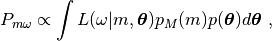
where  ,
,  are the prior
probabilities of model and parameters, respectively. The BioEM
software is used to perform the integrals in Eq. (1) over
orientation, PSF parameters, and center displacement using numerical
grid sampling. The remaining integrals over the intensity
normalization, offset, and noise are performed analytically following
ref. [1].
are the prior
probabilities of model and parameters, respectively. The BioEM
software is used to perform the integrals in Eq. (1) over
orientation, PSF parameters, and center displacement using numerical
grid sampling. The remaining integrals over the intensity
normalization, offset, and noise are performed analytically following
ref. [1].
The posterior probability of a single model given a set of images,
, becomes
(2)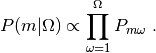
The main result of the BioEM software is the computation of Eq.
(2). This can be used for model comparison and discrimination
(e.g., to rank the best model) or to calculate the posterior
probability of a full set of models,  , following Eq. 2 of
ref. [1].
, following Eq. 2 of
ref. [1].
In this manual, it is assumed that the user has sufficient comprehension of the BioEM theory. Therefore, it is encouraged to read refs. [1][2] thoroughly.
Installation
Prerequisite programs and libraries
Before installation, there are several programs and libraries that should be preinstalled on the compute node. First check that the compiler is a modern C++ compiler which is OpenMP compliant. In the following, we give a brief explanation of the mandatory, and optional prerequisite programs.
Mandatory preinstalled libraries
- FFTW library (minimal version 3.3.3): is a subroutine library for computing the discrete Fourier transform. It is specifically used in BioEM, to calculate the convolution of the ideal image with the PSF, and the cross-correlation of the calculated image to the experimental image. FFTW can be downloaded from the webpage https://fftw.org/.
Optional preinstalled programs
The optional but encouraged to use programs for an easy compilation, and optimal performance, are described below:
- CMake (minimal version 2.6): is a cross-platform software for managing the build process of software using a compiler-independent method (i.e., creating a Makefile). CMake can be downloaded from https://cmake.org/.
- CUDA (minimal version 5.5): is a parallel computing platform implemented by the graphics processing units (GPUs) that NVIDIA produce. Thus, NVIDIA graphics cards are necessary for running BioEM with the CUDA implementation. For more information see https://nvidia.com/.
- MPI: Message Passing Interface is a standardized and portable message-passing system designed to function on a wide variety of parallel computers, with and without shared-memory. Any MPI platform (either openMPI or MPICH) can be used with BioEM. The minimal version of impi is 5.0.
- Git: is a system that is used for project development (see https://git-scm.com/). Git can be used to clone the BioEM software into a local directory.
After these programs are successfully installed on your compute node, it will be possible to install BioEM.
Note
It is recommended that the same compiler that is used to compile the libraries is also used to compile BioEM.
Download
The BioEM software can be cloned using git from https://github.com/bio-phys/BioEM with
git clone https://github.com/bio-phys/BioEM
A compressed directory of the BioEM software can be also directly downloaded from https://github.com/bio-phys/BioEM. After downloading the zip file, uncompress it by executing
unzip BioEM.zip
In the BioEM directory there are:
- the source code .cpp and .cu files.
- the include directory with corresponding header files.
- the copyright license, and README.md file.
- the CMakeLists.txt file that is necessary for installation with CMake (see below).
- the Quaternions directory that includes files with lists of quaternions that sample uniformly the rotational group SO3 (section Integration of orientations).
Download BioEM-tutorials
The BioEM tutorials can be cloned using git from https://github.com/bio-phys/BioEM-tutorials with
git clone https://github.com/bio-phys/BioEM-tutorials
A compressed directory of the BioEM tutorials can be also directly downloaded from https://github.com/bio-phys/BioEM-tutorials. After downloading the zip file, uncompress it by executing
unzip BioEM-tutorials.zip
In the BioEM-tutorials directory there are:
- the Tutorial_BioEM directory that includes the example files used in the tutorial (chapter Tutorial). Inside this directory, there is also a directory called MODEL_COMPARISON.
- the Cross-Validation_Tutorial directory that includes the example files used in the cross-validation tests.
Installing BioEM with CMake
The easiest installation of BioEM is done with the CMake program. CMake contains all the instructions to generate automatically a Makefile according to the specific architecture of the computing node, and the desired features of parallelization. CMake uses the CMakeLists.txt file. This file is provided in the uncompressed BioEM directory. The CMakeLists.txt has several modifiable options, that should be enabled/disabled (ON/OFF, respectively) according to the desired functionalities. The keywords for the modifiable options are shown in Table 1. These options can be enabled or disabled by executing cmake with
-D<optionname>=ON/OFF
For example, to turn on the compilation with CUDA run
cmake -DUSE_CUDA=ON CMakeLists.txt
It is also possible to modify these options directly in the CMakeLists.txt file. At the beginning of this file, the keywords and ON/OFF options are presented.
| <optionname> | Option |
|---|---|
USE_OPENMP |
Enable/Disable OpenMP |
USE_MPI |
Enable/Disable MPI |
USE_CUDA |
Enable/Disable CUDA |
PRINT_CMAKE_VARIABLES |
Printout CMake variables |
CUDA_FORCE_GCC |
Force of GCC as host compiler for CUDA part
(If standard host compiler is incompatible with CUDA)
|
Note
For certain architectures, an FindFFTW.cmake may be required to find the FFTW libraries. This file is included in the BioEM directory.
Steps for basic installation
- Create a build directory in the main BioEM directory, and access it by
mkdir build && cd build
- Run CMake with the desired options and the CMakeLists.txt file
cmake -D<optionname1>=ON -D<optionname2>=OFF ../CMakeLists.txt
- If this process is successful, a Makefile and CMakeFiles
directory should be generated. If this is not the case, enable the
variable
PRINT_CMAKE_VARIABLES, and re-run CMake with verbosity to debug. - After generating the Makefile, execute it
make
- If this process is successful a
bioEMexecutable should be generated.
For a simple test, run the BioEM executable
./bioEM
If the code runs successfully, the output on the terminal screen should be as shown in Listing 1.
 Command line inputs:
   --Modelfile       arg (Mandatory) Name of model file
   --Particlesfile   arg (Mandatory) Name of particle-image file
   --Inputfile       arg (Mandatory) Name of input parameter file
   --ReadOrientation arg (Optional) Read file name containing orientations
   --ReadPDB             (Optional) If reading model file in PDB format
   --ReadModelMRC        (Optional) If reading model file in MRC format
   --ReadMRC             (Optional) If reading particle file in MRC format
   --ReadMultipleMRC     (Optional) If reading multiple MRCs
   --DumpMaps            (Optional) Dump maps after they were read from particle-image file
   --LoadMapDump         (Optional) Read Maps from dump option
   --DumpModel           (Optional) Dump model after it was read from model file
   --LoadModelDump       (Optional) Read model from dump option
   --PrintCOORDREAD      (Optional) Print model coordinates
   --OutputFile      arg (Optional) For changing the outputfile name
   --help                (Optional) Produce help message
BioEM Input
In this chapter, we describe the BioEM input commands and keywords. BioEM has two main sources of input: from the commandline and from the input-parameter file. In the first section, we describe each commandline item from Listing 1. In the second section, we describe the keywords that should be specified in the input-parameter file. Lastly, we describe the specific formats of the model, particle-image, and input-parameter files that are used in the BioEM software.
Commandline input
The BioEM software requires a model, a set of experimental images and
a input-parameter file. The names of these files are passed to the
bioEM executable via the commandline, as well as their format
specifications. We now give a detailed description of the commandline
input items shown in Listing 1.
Model file
-
--Modelfile<arg>
The structural model is represented as spheres in 3-dimensional space. The position of the center of the sphere should be specified in the model file, as well as its corresponding radius and number of electrons. These spheres can represent atoms, coarse-grained residues or multi-scale blobs. The radius size approximately determines the resolution of the model. Spheres with radius less than the pixel size are projected on to a single pixel.
The name of the file containing the model has to be provided in the
commandline when bioEM is executed:
./bioEM --Modelfile arg
where arg is the model filename. The possible formats for the
model (pdb, text or starting from BioEM 2.1 mrc) are described
in section Formats for the model file.
Additional features to read the model in BioEM2.1
If one has to read the same model multiple times, the following options might be useful. The first time the model file is read, include in the commandline the keyword
-
--DumpModel
This will writeout a file model.dump containing the model in binary format, which will be useful for a faster re-reading.
To read the dumped model in binary format, use
-
--LoadModelDump
Note that the model.dump file should be in the same directory where
the code is executed. Using this last option, it is not necessary to
include --Modelfile in the commandline. See chapter
Tutorial for examples.
Particle-image file
The name of the experimental particle-image file is passed to the BioEM executable using the commandline:
-
--Particlesfile<arg>
where arg is the particle-image file name. The possible formats for
the particle-images (mrc or text) are described in section
Formats for the particle-images.
Additional features to read the particle-images
If one has to read the same particle-image set multiple times, the following options might be useful. The first time the particle-image file is read, include in the commandline the keyword
-
--DumpMaps
This will writeout a file maps.dump containing the particle-images in binary format, which will be useful for a faster re-reading.
To read the dumped maps in binary format, use
-
--LoadMapDump
Note that the maps.dump file should be in the same directory where
the code is executed. Using this last option, it is not necessary to
include --Particlesfile in the commandline. See chapter
Tutorial for examples.
Input-parameter file
BioEM has two sets of variables. One set describes the physical problem, like the number of pixels, and the parameter integration ranges. Another set describes the runtime configuration, which involves how to parallelize, whether to use a GPU, and some other algorithmic settings. The latter set does not change the output, but has a large influence on the compute performance. The two sets are treated differently, because the first set is related to the actual problem, while the second set belongs to the compute node where the problem is processed. For a detailed description of the performance variables see chapter Performance.
The physical parameters are passed via an input-parameter file that contains specific keywords for the physical constraints, and integration limits of the algorithm. The name of the input-parameter file is passed via the commandline:
-
--Inputfile<arg>
where arg is the filename.
In section Input of physical parameters, we describe in detail the keywords used in the input-parameter file.
Orientations from a file
In BioEM there is an option to read the orientations of a model directly from a file, instead of calculating them in the code (see also section Integration of orientations). This option provides more flexibility to perform the integral over the orientations.
For this feature use the following commandline keyword
-
--ReadOrientation<arg>
where arg is the name of the file containing the list of
orientations. The format for the orientations (Euler angles or
quaternions) is described in section Formats for the orientations file.
BioEM output
By default, the main BioEM output file is called
Output_Probabilities
To change the name of the output file use the following commandline keyword
-
--OutputFile<arg>
where arg is the desired name of the output file. This file contains
the logarithm of the posterior probability of the model to each
individual experimental image and the parameter set that gives a maximum
of the posterior (see section Output format for its format).
To check that model coordinates, radius and density are read correctly, inspect the COORDREAD file that can be generated using the following commandline keyword
-
--PrintCOORDREAD
Note that printing of COORDREAD file has become optional starting from BioEM2.1, while in the older BioEM versions, the output file was always generated.
Input of physical parameters
Up to now, we have seen several commandline inputs that can be used in BioEM. We now focus on the input of the physical parameters that are necessary for the BioEM computation and are read from inside the input-parameter file. These parameters describe the physical constraints of the algorithm, such as the integration ranges and grid points, and are passed using specific keywords in the this file (see also section Input-parameter file).
Micrograph parameters
Mandatory inputs for the description of the experimental particle-image are
PIXEL_SIZE (float)Pixel size in
of the experimental micrograph.
NUMBER_PIXELS (int)We assume a square particle-image. Here,
(int)is the number of pixels in each dimension, e.g., for a particle-image of 220 x 220 pixels, then(int)= 220.
In the BioEM calculation, the integration over the model orientations, PSF parameters, and center displacement are performed numerically. To do so, one needs to define the integration ranges, and grid spacing for each parameter. These quantities depend on the experimental conditions, such as defocus range, and thus should be specified by the user.
Integration of orientations
There are two ways to describe the orientation of the model in 3D space: with the Euler angles or with quaternions.
- Euler Angles. The Euler angles are
 , and
represent a sequence of three elemental rotations about the axes of a
coordinate system. We use the reference rotations
, and
represent a sequence of three elemental rotations about the axes of a
coordinate system. We use the reference rotations
 , such that the first rotation is around the
-axis by an angle
, such that the first rotation is around the
-axis by an angle  , the second rotation is
around the
, the second rotation is
around the  -axis by an angle
  , and a last
rotation is again around the -axis by an angle
, and a last
rotation is again around the -axis by an angle
 .
. - Quaternions. The orientation of a rigid body can also be described
with quaternions. A set of quaternions is a four-dimensional vector
over the real numbers (
 ,
,  ,
,  ,
,
 ) each within
 ![[-1,1]](_images/math/49a47d5b84588d4baba9dd7f7e2c5f4251aa643a.png) such that
such that
 .
.
There are several ways to sample the space of Euler angles or quaternions. We importantly remark that not all possibilities sample uniformly the group of rotations in 3D space (SO3), which is crucial to perform a fast and accurate integration of uniformly distributed model orientations.
Uniform sampling of SO3
To uniformly sample SO3, we recommend using a list of quaternions
generated with the successive orthonormal images method from
ref. [3]. In the directory Quaternions, we
provide lists of quaternions that have been generated using this
method. Here, it is necessary to follow section Orientations from a file because
a list of quaternions is read from a separate file. To use quaternions
the keyword USE_QUATERNIONS in the input-parameter file is
also required.
Non-uniform sampling
It is also possible to have trivial grid-sampling of the Euler angles or quaternions:
Grid-sampling of the Euler Angles (
): Sampling of the full Euler angle space within an uniform
cubic-grid: ![\alpha \in [-\pi,\pi]](_images/math/deb7224ee43781111b483b7b66cb60b285c05472.png) ,
, ![\cos(\beta) \in
[-1,1]](_images/math/f3849074b51fe0ee5211b0365927d818c94c8633.png) and
and ![\gamma \in [-\pi,\pi]](_images/math/bbe7ab018b7d272abb240bcc668462940485c7ab.png) . Here one needs to
provide the number of grid points in , and
. Here one needs to
provide the number of grid points in , and
 . By default, the grid spacing of Euler angle
will be the same as that of . The
keywords in the parameter file are
. By default, the grid spacing of Euler angle
will be the same as that of . The
keywords in the parameter file are-
GRIDPOINTS_ALPHA (int)
-
GRIDPOINTS_BETA (int)
where
(int)is the number of grid points.Note
For an optimal grid spacing, it is recommended that
GRIDPOINTS_ALPHA~ 2*GRIDPOINTS_BETA.-
Grid-sampling of quaternions: With BioEM it is also possible to generate a grid in quaternion space. One should provide the keywords
-
USE_QUATERNIONS
-
GRIDPOINTS_QUATERNION (int)
where
(int)is the grid spacing in each dimension.-
Non-uniform sampling of orientations from a file: We note that with the option of reading the orientations from a file (section Orientations from a file) the user has great freedom to sample also non-uniformly the orientation space (for example around a given orientation, see Example: model comparison using BioEM).
Integration of the PSF parameters
To take into account the interference effects in the experiment, we convolute the ideal image from the model with the PSF. In practice, we use its Fourier-space equivalent, which is the multiplication the contrast transfer function (CTF) and envelope function. An approximate expression for the CTF is

where  is the radial spatial frequency, and
 with
with  is the electron
wavelength, and
is the electron
wavelength, and  is the defocus. Parameter
![A \in [0,1]](_images/math/5bfe9ae86d3a2140e4b6ad1a47f9194f249140a2.png) establishes the contributions of the cosine and sine
components.
establishes the contributions of the cosine and sine
components.
The envelope function is
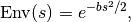
where parameter  controls the Gaussian width and modulates the
CTF.
controls the Gaussian width and modulates the
CTF.
To calculate the BioEM posterior probability, we integrate numerically
the three parameters , and  . To do
so, one should include in the input-parameter file the keyword for each
parameter, its integration limits, and number of grid points:
. To do
so, one should include in the input-parameter file the keyword for each
parameter, its integration limits, and number of grid points:
Parameter – (start) – (end) – (gridpoints)
CTF_DEFOCUS (float) (float) (int)
CTF_B_ENV (float) (float) (int)
CTF_AMPLITUDE (float) (float) (int)
The defocus, , should be in units of  m,
and in Å
m,
and in Å . The amplitude parameter is
adimensional within
. The amplitude parameter is
adimensional within ![[0,1]](_images/math/62f34fae2b08036cedb90a3ebf47f74a61dcb1be.png) . The default value of the electron
wavelength is 0.019688, which corresponds to a
. The default value of the electron
wavelength is 0.019688, which corresponds to a  microscope. To change this value use the keyword
ELECTRON_WAVELENGTH (float)
where (float) should be in .
Integration of center displacement
The integration of the particle center is done over a square and uniform grid. The particle, along both directions, is translated from its center up to a maximum distance (max displ.). Users should provide this maximum displacement and the grid spacing in units of pixels.
The keyword in parameter file is:
Parameter - (max displ.) - (grid-space)
DISPLACE_CENTER (int) (int)
If [DISPLACE_CENTER 10 2], the integration will be done along
within ![[x_c-10,x_c+10]](_images/math/d3beaa59f851318ec3fb18d2c3ca9319be2ac767.png) (where
(where  is the
center), and
is the
center), and ![[y_c-10,y_c+10]](_images/math/4515a56a79488be77208aa541a86abf14d457fac.png) along
along  , with sampling
every 2 pixels.
, with sampling
every 2 pixels.
The integration over the normalization, offset and noise are carried out analytically. See Supplementary Information of ref. [1].
Priors
Uniform model prior probability: To include a uniform model prior use the following keyword in the input-parameter file
-
PRIOR_MODEL (float)
where
(float)is the value of the model’s prior.-
Prior for orientations: It is possible to assign prior probabilities for each orientation. The keyword
-
PRIOR_ANGLES
allows to read the prior of each orientation from the input file of orientations (see section Orientations from a file). An extra column of format “%12.6f” should be added in the orientations-file, which indicates the value of the prior probability for each orientation.
-
Prior for
envelope parameter: To avoid full loss of
the high-frequency components in Fourier space, the code utilizes a
Gaussian prior on the envelope parameter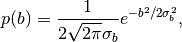
where
 is the Gaussian width. By default the
Gaussian prior is centered at zero, and
is the Gaussian width. By default the
Gaussian prior is centered at zero, and  , to
modify the width include in the input-parameter file the keyword
, to
modify the width include in the input-parameter file the keyword-
SIGMA_PRIOR_B_CTF (float)
where
(float)is the desired. See also the
supporting information of ref. [2].-
Prior for
defocus parameter: BioEM implements a
Gaussian prior on the defocus parameter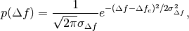
where
 is the Gaussian width and
 is the Gaussian center. By default
 m, and
  m. To modify these values include in the
input-parameter file the keyword
m. To modify these values include in the
input-parameter file the keyword-
SIGMA_PRIOR_DEFOCUS (float)
where
(float)is the desired, and-
PRIOR_DEFOCUS_CENTER (float)
to change the Gaussian center
. See also the
supporting information of ref. [2].-
Prior for
amplitude parameter: BioEM implements a
Gaussian prior on the amplitude parameter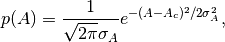
where
 is the Gaussian width and
  is
the Gaussian center. By default
is
the Gaussian center. By default  , and
, and
 . To modify these values include in the input-parameter
file the keyword
. To modify these values include in the input-parameter
file the keyword-
SIGMA_PRIOR_AMP_CTF (float)
where
(float)is the desired, and-
PRIOR_AMP_CTF_CENTER (float)
to change the Gaussian center
.-
Posterior probability as a function of orientations
One can write out the log-posterior as a function of each orientation. In this case, the integration is performed over the CTF parameters, particle-center, normalization, offset and noise, but not over the orientations. The keyword in parameter file is
WRITE_PROB_ANGLES (int)
With this feature there is an additional output file
ANG_PROB where (int) orientations with highest posterior
are written. The orientations in this file are sorted in decreasing log-posterior
order.
Overview of keywords for the input-parameter file
In the following, we provide a list of the possible keywords read from the input-parameter.
BioEM posterior probability computation:
PIXEL_SIZE(float): Micrograph pixel size in Å.NUMBER_PIXELS(int): Assuming a square particle-image, it is the number of pixels along an axis. This should coincide with the number of pixels read from the micrograph.CTF_DEFOCUS(float) (float) (int): (CTF integration) Grid sampling of CTF defocus,. Units of
micro-meters. (float) (float)are the starting and ending limits, respectively, and(int)is the number of grid points.CTF_B_ENV(float) (float) (int): (CTF integration) Grid sampling of envelope parameter. Units of Å. (float) (float)are the starting and ending limits, respectively, and(int)is the number of grid points.CTF_AMPLITUDE(float) (float) (int): (CTF integration) Grid sampling of the CTF amplitude, (adimensional
![\in [0,1]](_images/math/0268e0a93e47bc316c3d24060f782557873cd7bd.png) ).
). (float) (float)are the starting and ending limits, respectively, and(int)is the number of grid points.DISPLACE_CENTER(int) (int): (Integration of particle center displacement) Sampling within a square grid. Units of pixels.(int) (int)are the maximum displacement from the center in both directions, and the grid spacing, respectively.
Optional keywords:
GRIDPOINTS_ALPHA(int): (Integration of orientations, mandatory if quaterionions or –ReadOrientation are not used) Number of grid points used in the integration over Euler angle. Here a cubic grid in Euler angle
space is performed. The integral over Euler angle is
identical to that of .GRIDPOINTS_BETA(int): (Integration of orientations, mandatory if quaterionions or –ReadOrientation are not used) Number of grid points used in the integration over![\cos(\beta) \in [-1,1]](_images/math/cd022a9fdeefb83bde23bae47c3de7ae045f8d8d.png) .
.USE_QUATERNIONS: (Integration of Orientations) If using quaternions to the describe the orientations. Recommended for uniformly sampling of with the quaternions lists
available in the Quaternions directory.
with the quaternions lists
available in the Quaternions directory.GRIDPOINTS_QUATERNION(int): (Integration of Orientations) For a hypercubic grid quaternion sampling. Each quaternion is within. (int)is the number of grid points per dimension.ELECTRON_WAVELENGTH(float): To change the default value of the electron wavelength(float)used to calculate the CTF phase with the defocus. Default 0.019688.PRIOR_MODEL(float): Prior probability of model. Default 1.PRIOR_ANGLES: To read the prior of each orientation in the input file of orientations.SIGMA_PRIOR_B_CTF(float): To change the Gaussian width of the prior probability of the CTF envelope parameter
(section Priors). Default 100 Å.SIGMA_PRIOR_DEFOCUS(float): To change the Gaussian width of the prior of the defocus
(section Priors). Default 1 m.PRIOR_DEFOCUS_CENTER(float): To change the Gaussian center of the prior of the defocus (section
Priors). Default 3 m.SIGMA_PRIOR_AMP_CTF(float): To change the Gaussian width of the prior of the amplitude (section
Priors). Default 0.3.PRIOR_AMP_CTF_CENTER(float): To change the Gaussian center of the prior of the amplitude (section
Priors). Default 0.NO_MAP_NORM: Condition to not normalize to zero mean and unit variance the input maps.WRITE_PROB_ANGLES(int): To write out the posterior as a function of the best(int)orientation.
File formats
Formats for the model file
There are two types of model file formats that are read by BioEM:
Text file: A simple text file with format “%f %f %f %f %f”. The first three columns are the coordinates of the sphere centers in
, the fourth column is the radius in , and the
last column is the corresponding number of electrons (which can be non-integer).(Format:
x — y — z — radius — number electrons).This format is useful for all atom, mixed or coarse-grained representations of the density maps.
pdb file: BioEM reads the C
 atom positions with
their corresponding residue type from standard pdb files. A
residue is modeled as a sphere, centered at the C,
with van-der-Waals radii and number of electrons corresponding to
the specific amino acid type (as in
ref. [1]). To read pdb files the following
commandline keyword is needed (related to section Model file):
atom positions with
their corresponding residue type from standard pdb files. A
residue is modeled as a sphere, centered at the C,
with van-der-Waals radii and number of electrons corresponding to
the specific amino acid type (as in
ref. [1]). To read pdb files the following
commandline keyword is needed (related to section Model file):-
--ReadPDB
-
mrc file: BioEM reads the intensities from standard mrc files. The pixel size is read from the Input-parameter file (Input-parameter file) To read mrc files the following commandline keyword is needed (related to section Model file):
-
--ReadModelMRC
-
Formats for the particle-images
Two format options are allowed for the the particle-image file:
Text file: Data are formatted as “%8d%8d%16.8f” where the first two columns are the pixel indexes, and the third column is the intensity at that pixel. Multiple particles are read in the same file with the separator
PARTICLE. Pixel indexes should start at 0, and all pixels should be included..mrc file: BioEM also reads standard .mrc particle-image files. To do so, the additional commandline keyword is needed:
-
--ReadMRC
-
If reading multiple mrc files, the name of the file containing the list of all the mrc files should be provided. The additional command is required:
-
--ReadMultipleMRC
Example:
--Particlesfile LIST --ReadMRC --ReadMultipleMRC
LISTis the name of the file containing the list of names of the multiple mrc files.Note
When mrc particles are read, by default the intensities are normalized to zero average and unit standard deviation. Use the keyword
NO_MAP_NORMin the input-parameter file to unset this default.-
Formats for the orientations file
Related to sections Orientations from a file and Integration of orientations. The format for the orientations file is described in the following:
- The first row of the file should have
(int)equal to the total number of orientations. - The orientations can be described with Euler angles, or with
quaternions:
- Euler angles. These are Euler angles
in radians, which representing three rotations about axis
 . The format for the file containing the Euler
angles is “%12.6f%12.6f%12.6f”, ordered as
, respectively.
. The format for the file containing the Euler
angles is “%12.6f%12.6f%12.6f”, ordered as
, respectively. - Quaternions. A set of quaternions is a four-dimensional vector
over the real numbers (, , ,
) each within . The format for this
file containing the quaternions should be
“%12.6f%12.6f%12.6f%12.6f”, ordered as , ,
, and , respectively. To use quaternions
the keyword
USE_QUATERNIONSshould be placed in the input-parameter file.
- Euler angles. These are Euler angles
- Prior for orientations. Its possible to assign prior probabilities to each orientation. To do so, one should add at the end of each line an extra column (of format “%12.6f”) that indicates the value of the prior probability for each orientation.
Output format
The main BioEM output file is called Output_Probabilities by
default. Its name can be changed using the commandline
--OutputFile as described in section BioEM output. This file
contains the logarithm of the posterior probability of the model to
each individual experimental image.
RefMap [number Particle Map] LogProb [ln(P)]
It also reports the parameter grid values that give a maximum value of the posterior probability.
RefMap [number Particle Map] Maximizing Param: [Orientation] [PSF parameters] [center displacement] [norm] [offset]
Important remark: The posterior probability is not normalized. Thus,
it is always recommended to compare  of different
models or relative to noise as in ref. [1]
(see also section Example: model comparison using BioEM).
of different
models or relative to noise as in ref. [1]
(see also section Example: model comparison using BioEM).
Before executing a production run, it is recommended to check that the values of the log-posterior are finite, and the parameters that give a maximum of the posterior are in a reasonable range (e.g., not at the borders of the integration limits).
Optional outputs
The optional output files for BioEM are:
COORDREADThis file used to be generated always, but in the newer BioEM versions it is generated only when the option
--PrintCOORDREADis used. This output file allows to check that the model coordinates, radius and density are read correctly. It is reported in the following format
Text --- Number ---- x ---- y ---- z ---- radius ---- number of electron

.. outpar:: ANG_PROB
.. object:: ANG_PROB

  Related to section :ref:`angprob`. This file has the posterior
  probabilities for each orientation, which was specified with the
  keyword :inpar:`WRITE_PROB_ANGLES` in the parameter inputfile.
  For the Euler angles, the format of the output file is

.. code-block:: bash

   [Map number -- alpha -- beta -- gamma -- log Probability]

For the quaternions, its format is

.. code-block:: bash

   [Map number -- q1 -- q2 -- q3 -- q4 -- log Probability]
Performance
The BioEM performance variables enhance or modify the code’s computational performance without modifying the numerical results. They should be tuned for the specific computing node characteristics where BioEM is executed. They are passed via environment variables using the bash scripting language.
In the following chapter, we explain the types of parallelization used within the BioEM software, list all relevant environment variables, and provide some suggestions for runtime configurations in different situations.
Ways of parallelization
BioEM compares various projections of a model to a set of reference particle-images. As explained in section Theoretical background the model is first projected along a given angular orientation, then it is convoluted with the PSF, next it is shifted by a certain number of pixels to account for the center displacement, and finally this modified projection is compared to a reference particle-image.
From a computational complexity perspective, the performance depends mostly on the number of angular orientations relative to the number experimental images. If there are many experimental images and many orientations then the comparison of the calculated projection to all the experimental images is by far the most time consuming part. However, if there are few experimental images and many orientations, the comparison part is not the time-limiting step.
BioEM 2.0 has been optimized for both CPU and GPU performance according to two different scenarios:
- Many orientations versus many experimental images
- Many orientations versus few experimental images
Because the optimal parallelization scheme changes depending on the previous conditions, we address each item separately.
Many orientations vs. many experimental images
BioEM facilitates the comparison of many orientations to many experimental images using an all model projections to an all particle-image comparison through a nested loop.
For this case, the following external variable modulates the BioEM optimization algorithm:
export BIOEM_ALGO=1
As shown in Fig. 2 of ref. [2], in the
BIOEM_ALGO=1 the outermost loop is over the
orientations and the inner most loop iterates over all particle-images
and center displacements.
Parallelization
There are multiple dimensions for parallelization:
MPI: BioEM uses MPI to parallelize over the orientations in the outermost loop. In this case the probabilities for all particle-images / PSF kernels / center displacements are calculated for a certain subset of orientations by each MPI process. Afterward, the probabilities computed by every MPI process are reduced to the final probabilities. If started via
mpirun, BioEM will automatically distribute the orientations evenly among all MPI processes.OpenMP: BioEM can use OpenMP to parallelize over the particle images in the innermost loop. As processing of these particle-images is totally independent, there is no synchronization required at all. BioEM will automatically multithread over the particle-images. The number of employed threads can be controlled with the standard
export OMP_NUM_THREADS=[x]
environment variable for OpenMP, where
[x]is the number of OpenMP threads.Graphics Processing Units (GPUs): BioEM can use GPUs to speed up the processing. In this case, the innermost loop over all particle-images, and with all center displacements, is processed by the GPU. The projections and the PSF convolutions are still processed by the CPU. This process is pipelined such that the CPU prepares the next projections, and PSF convolutions while the GPU calculates the probabilities to all particle-images for the previous calculated projections. Hence, this is a horizontal parallelization layer among the particle images with an additional vertical layer through the pipeline. Usage of GPUs must be enabled with the
export GPU=1
environment variable. One BioEM process will always only use one GPU, by default the fastest one. A GPU device can be explicitly configured with the environment variable:
export GPUDEVICE=[x]
Multiple GPUs can be used through MPI. In this case, every GPU will process all particle-images but calculate the probabilities only for a subset of the orientations (see description of MPI above). Selection of GPU devices for each process must be carried out by
export GPUDEVICE=-1
In this case the MPI process with rank N on a system with G GPUs will take the GPU with ID (N % G). This option is mandatory when using MPI.
GPU / CPU combined processing: Besides the pipeline approach described in the previous point, which employs the CPU for creating the calculated image, and the GPU for calculating the likelihood to all particle-images, there is also the possibility to split the set of particle-images among the CPU and the GPU. This is facilitated by the environment variable
export GPUWORKLOAD=-1
that automatically sets the percentage of particle-images processed by the GPU.
It is also possible to not use this autotuning option but to set a static value provided by the user
export GPUWORKLOAD=[x]
where
 provides the x% of particles processed by
the GPU. However, the autotuning option is set by default.
provides the x% of particles processed by
the GPU. However, the autotuning option is set by default.In an optimal situation the CPU will:
- Issue a GPU kernel call such that the GPU calculates the probabilities for x% of the particle-images for the current orientation and convolution.
- Process its own fraction of (100-x)% of the particle-images in parallel to the GPU.
- Afterward, finish the preparation of the next orientation and PSF convolution before the GPU has finished calculating the probabilities for the current orientation and PSF convolution.
Multiple Projections/Convolutions at once via OpenMP: BioEM can prepare the projections of multiple orientations and convolutions at once using OpenMP. The benefit compared to the pure OpenMP parallelization over the particle images, however, is tiny, while the memory requirements are drastically increased. This is relevant if MPI is not used, OpenMP is used, GPU is not used, and if the number of reference particle-image is small. The number of projections at once is determined by the environment variable
export BIOEM_PROJ_CONV_AT_ONCE=[x]
where
[x]is the number of projections that will be calculated simultaneously.Fourier-algorithm to process all center displacements in parallel: BioEM uses as default the Fourier-algorithm to calculate the cross-correlation. The Fourier-algorithm automatically takes all displacements into account without having to loop over them. Hence, its runtime is almost independent from the number of center displacements (see ref. [2]).
Parallelization on only CPUs
For parallelization over the CPU cores:
One can use MPI with as many MPI processes as there are CPU cores
 nodes, and with
 OMP_NUM_THREADS=1. In this case, the parallelization is done only over the orientations.On a single node, one can use OpenMP to parallelize over the particle images, and optionally using the environmental variable
BIOEM_PROJ_CONV_AT_ONCE=[x]to increase number of projections/convolutions processed in parallel.One can combine both MPI and OpenMP, as shown in ref. [2]. For instance, on a single node,
OMP_NUM_THREADS=[x]can be set tox = 1/4 N, whereNis the number of CPU cores on the system, and BioEM can be called withmpirun, and 4 MPI processes. In this case, four orientations are processed in parallel using MPI, andxparticle-images are processed in parallel using OpenMP.If multiple nodes are used MPI is mandatory, and should be combined with OpenMP. Optimal work distribution will depend on the number of orientations (parallelization with MPI) compared to the number of particle-images (parallelization with OpenMP).
Note
To find the optimal performance setup for only CPUs, it is recommended to try both BioEM algorithms
BIOEM_ALGO=1andBIOEM_ALGO=2with different combinations of the options described.
Parallelization on CPUs and GPUs
Naturally, different methods of parallelization can be combined with the GPU:
- One can combine MPI with the GPU algorithm to use multiple GPUs at once. The number of MPI processes has to be equal to the number of available GPUs.
- One can use GPUs and CPU cores jointly to calculate the
probabilities for all particle-images with OpenMP and the
GPUWORKLOAD=-1autotunning variable. For more than one GPU, MPI must be employed. In this case, the number of MPI processes must match the number of GPUs. So it is important to combine MPI, and OpenMP inside one node in order to use all CPU cores.
Examples of possible ways of parallelization are shown in Fig. 5 and 6 of ref. [2] for the FRH protein complex system.
Many orientations vs. few experimental images
BioEM2.0 has been optimized to treat many orientations and few experimental images using GPUs and CPUs. For this case, the following external variable modulates the BioEM algorithm:
export BIOEM_ALGO=2
In this algorithm, the parallelization for GPU is now done on a lower level: the GPU (or OpenMP for the only CPU case) processes the center displacements, whilst the CPU with MPI processes the orientations and with OpenMP the projections and convolutions. Hence, there is more parallelism and better performance for the GPU for this case.
Parallelization
We present the different parallelization options when using the
BIOEM_ALGO=2:
- MPI: Similarly as with
BIOEM_ALGO=1(section Many orientations vs. many experimental images) MPI is used to parallelize over the orientations in the outermost loop. - OpenMP: With
BIOEM_ALGO=2theBIOEM_PROJ_CONV_AT_ONCEis by default equal toOMP_NUM_THREADS. However,BIOEM_PROJ_CONV_AT_ONCEcan also be modified as described above. Importantly, forBIOEM_ALGO=2the contribution ofBIOEM_PROJ_CONV_AT_ONCEis significant. These OMP threads are used to work in parallel on the projections, the convolutions, and if GPU is disabled on the center displacements and comparisons. - Graphics Processing Units (GPUs): For
BIOEM_ALGO=2the loop over center displacements can be processed by the GPU. The projections and convolutions are still processed by the CPU. The GPU environment variables areGPU=1to use the GPU andGPUDEVICE=[x]to select the GPU device. WithGPUDEVICE=-1the GPU is automatically selected. Note thatGPUWORKLOADis always100, meaning that all center displacements are always processed by GPU. - Fourier-algorithm to process all center displacements in parallel:
For
BIOEM_ALGO=2, the Fourier-algorithm is also default and always used.
Parallelization on only CPUs
For BIOEM_ALGO=2 and only CPUs:
- One can use MPI with as many MPI processes as there are CPU cores
nodes and with
OMP_NUM_THREADS=1. In this case, the parallelization is done only over the orientations . - On a single node, one can use OpenMP with
OMP_NUM_THREADS=[x]to parallelize over the projections, convolutions and center displacements (by default using alsoBIOEM_PROJ_CONV_AT_ONCE). - One can combine both MPI and OpenMP where MPI runs over the
orientations and OpenMP over the projections, convolutions and
center displacements. For instance, on a single node,
OMP_NUM_THREADS=[x]can be set tox = 1/4 N, whereNis the number of CPU cores on the system, and BioEM can be called withmpirun, and 4 MPI processes. - If multiple nodes are used MPI is mandatory, and should be combined with OpenMP. Optimal work distribution will depend on the specifications of the nodes, and the number of orientations compared to the number of particle-images.
Note
To find the optimal performance setup for only CPUs, it is
recommended to try both BioEM algorithms BIOEM_ALGO=1 and BIOEM_ALGO=2 with different combinations
of the options described.
Parallelization on CPUs and GPUs
For BIOEM_ALGO=2, different methods of GPU and CPU
parallelization can be combined:
- One can combine MPI with the GPU algorithm to use multiple GPUs at once. The number of MPI processes has to be equal to the number of available GPUs.
- One can use GPUs and CPU cores jointly. MPI will parallelize over the orientations, OpenMP can parallelize over the projections and the GPU over the convolutions and center displacements. The number of MPI processes must match the number of GPUs. So it is important to combine MPI and OpenMP inside one node in order to use all CPU cores.
Note on the numerical results
BioEM2.0 combines float and double-precision variables. Float precision is used for most variables within the code, which significantly speeds-up the calculations (see [2]). By contrary, the posterior probability is handled in double precision to maintain a high numerical accuracy. Nonetheless, we note that there could be a minimal numerical difference in the computed probabilities, depending whether CPUs, GPUs or a combination of both is used. This is coming from the different results and rounding errors on different hardware and different underlying libraries, thus it is hard to avoid it. However, in all practical cases this minimal discrepancies can be considered negligible; much smaller than the uncertainties of the numerical integrations.
List of environment variables
-
BIOEM_ALGO¶ (Default: 1) Set to 1 to enable the BioEM algorithm optimized for many orientations versus many experiment images computations. Set to 2 to enable the BioEM algorithm optimized for many orientations versus few experiment images computations.
-
GPU¶ (Default: 0) Set to 1 to enable GPU usage, set to 0 to use only the CPU.
-
GPUDEVICE¶ (Default: fastest) Only relevant if
GPU=1.- If this is not set, BioEM will autodetect the fastest GPU. Only possible if MPI is not used.
- If
x >= 0, BioEM will use GPU numberx. Only possible if MPI is not used. - If
x = -1, BioEM runs withNMPI threads, and the system hasGGPUs, then BioEM will use GPU with number (N % G). The idea is that one can place multiple MPI processes on one node, and each will use a different GPU. For a multi-node configuration, one must make sure that consecutive MPI ranks are placed on the same node, i.e., four processes on two nodes (node0 and node1) must be placed as (node0, node0, node1, node1) and not as (node0, node1, node0, node1), because in the latter case only 1 GPU per node will be used (by two MPI processes each).
-
GPUWORKLOAD¶ (Default: -1 for
BIOEM_ALGO=1and fixed to 100 forBIOEM_ALGO=2) Only relevant ifGPU=1. This defines the fraction of the workload in percent. To be precise: the fraction of the number of particle-images processed by the GPU. The remaining particle-images will be processed by the CPU. ForBIOEM_ALGO=1, if set to -1 the autotuning option will automatically select the ideal % of particles processed by the GPU. ForBIOEM_ALGO=2it is fixed toGPUWORKLOAD=100.
-
GPUASYNC¶ (Default: 1) Only relevant if
GPU=1. This uses a pipeline to overlap the processing on the GPU, the preparation of projections and convolutions on the CPU, and the DMA transfer. There is no reason to disable this except for debugging purposes.
-
GPUDUALSTREAM¶ (Default: 1) Only relevant if
GPU=1. If this is set to 1, the GPU will use two streams in parallel. This can help to improve the GPU utilization. Benchmarks have shown that there is a very little positive effect by this setting, as utilization of GPU is already high.
-
BIOEM_CUDA_THREAD_COUNT¶ (Default: 256 for
BIOEM_ALGO=1and 512 forBIOEM_ALGO=2) Only relevant ifGPU=1. This variable can explicitly select the number of CUDA threads. Different inputs and algorithms might need different number of threads for an optimized performance, but also to respect hardware (memory) limits of a GPU device.
-
OMP_NUM_THREADS¶ (Default: Number of CPU cores) This is the standard OpenMP environment variable to define the number of OpenMP threads. It can be used for profiling purposes to analyze the scaling. It can be set to
x=1to use MPI exclusively or to other values for a mixed MPI / OpenMP configuration.
-
BIOEM_PROJ_CONV_AT_ONCE¶ (Default: 1 for
BIOEM_ALGO=1and=OMP_NUM_THREADSforBIOEM_ALGO=2) This defines the number of projections and convolutions prepared at once. OpenMP threads (whose number is defined byOMP_NUM_THREADSenvironment variable) are used to prepare these projections and convolutions in parallel. ForBIOEM_ALGO=1BIOEM_PROJ_CONV_AT_ONCE=[x]is mostly relevant, if OpenMP is used, no GPU is used, and/or the number of reference particle-image is very small. ForBIOEM_ALGO=2its contribution is important.
-
BIOEM_DEBUG_BREAK¶ (Default: deactivated) This is a debugging option. It will reduce the number of projection and PSF convolutions to a maximum of
xboth. It can be used for profiling to analyze scaling, and for fast sanity tests.
-
BIOEM_DEBUG_NMAPS¶ (Default: deactivated) As
BIOEM_DEBUG_BREAK, with the difference that this limits the number of reference particle-images to a maximum ofx.
-
BIOEM_DEBUG_OUTPUT¶ (Default: 0) Change the verbosity of the output. Higher means more output, lower means less output.
x=0: Stands for no debug output.x=1: Limited timing output.x=2: Standard timing output showing durations of projection, convolution, and cross-correlation comparison. This adds successively more extensive output.
Default environment variables
With BioEM2.0 the Fourier-algorithm [2]
is always used. This implies that the GPU algorithm is by default
GPUALGO=2 (defined in BioEM1.0). It has been shown that for
realistic cases, where the particle center is an unknown parameter, the
Fourier-algorithm outperforms all other algorithms. Because of this, we
have selected it to be permanently default.
Suggestions for runtime configurations
Default Settings
It is recommended that the following settings should be left at theirs
defaults: GPUASYNC (Default 1), GPUDUALSTREAM
(Default 1).
Profiling
For profiling one can limit the number of orientations, projections
and particle-images for example using BIOEM_DEBUG_BREAK and
BIOEM_DEBUG_NMAPS. However, for accurate estimations, it is
recommended to keep the proportion of orientations to particle-images
the same as in the actual application. Also a good choice is
BIOEM_DEBUG_OUTPUT=2 to get the timing of each
projection, convolution and comparison. For a larger number of
particle-images it might make sense to switch to
BIOEM_DEBUG_OUTPUT=1.
Production run: Many orientations vs. many experimental images
On only CPUs
BIOEM_ALGO=1to select the BioEM algorithm 1 that optimizes the computation of many orientations to many particle images.BIOEM_DEBUG_OUTPUT=0can reduce the size of the text output.BIOEM_PROJ_CONV_AT_ONCE=[x]may have a positive effect. The memory footprint increases withx, so it should not be too large. For best performance, choose a multiple of the number of OpenMP threads.On a single node, one should use OpenMP parallelization for many particle-images and few orientations; and MPI parallelization for few particle-images and many orientations. Assume a system with
NCPU cores, the command for the first would beBIOEM_PROJ_CONV_AT_ONCE=[4*N] OMP_NUM_THREADS=[N]and for the second
OMP_NUM_THREADS=1 ; mpirun -n [N]For a medium number of particle-images and orientations, a combined MPI / OpenMP configuration can be better.
Example: Assume 20 CPU cores, possible options would be (among others):
20 MPI processes with 1 OMP thread each:
OMP_NUM_THREADS=1 mpirun -n 2010 MPI processes with 2 OMP threads each:
OMP_NUM_THREADS=2 mpirun -n 104 MPI processes with 5 OMP threads each:
OMP_NUM_THREADS=5 mpirun -n 42 MPI processes with 10 OMP threads each:
OMP_NUM_THREADS=10 mpirun -n 2
The best configuration has to be checked by the user. But in any case, one should make sure that the number of MPI processes times the number of OMP threads per process equals the number of (virtual) CPU cores. Importantly, one should also compare the timings from
BIOEM_ALGO=1orBIOEM_ALGO=2with the different configurations.
On combined CPUs and GPUs
BIOEM_ALGO=1to select the BioEM algorithm 1 that optimizes the computation of many orientations to many particle images.BIOEM_DEBUG_OUTPUT=0can reduce the size of the text output.BIOEM_PROJ_CONV_AT_ONCE=[x]may have a positive effect. However, the memory footprint increases withx, it this can be a limiting factor for GPUs. Therefore, it is usually enough to keep the defaultBIOEM_PROJ_CONV_AT_ONCE=1, unless the number of particle images is small (in which case one should consider theBIOEM_ALGO=2algorithm anyway).GPU=1should be used if a GPU isavailable. Performance wise, one Titan GPU corresponds roughly to 20 cores at 3 GHz.
GPUWORKLOAD=-1for autotuning of the optimal workload balance.If a system offers multiple GPUs, all GPUs should be used. This must be accomplished via MPI. In this case, the number of MPI processes per node must match the number of GPUs per node. There are different ways to make sure every MPI process uses a different GPU (as discussed in the GPU paragraph of section Ways of parallelization). Assuming the MPI processes are placed such, that consecutive MPI ranks are placed on one node, one can use the
GPUDEVICE=-1setting. This is assumed here. Let us assume an example ofNnodes withCCPU cores each andGGPUs each. The following command will use all GPUs, and ignore the CPUs:OMP_NUM_THREADS=1 GPU=1 GPUDEVICE=-1 mpirun -n [N*G]One can use all the CPU cores as well as the GPUs. A combined MPI / OpenMP setting as discussed previously must be used, under the constraint that the number of MPI processes matches the number of GPUs:
OMP_NUM_THREADS=[C/G] GPU=1 GPUDEVICE=-1 mpirun -n [N*G]
Production run: Many orientations vs. few experimental images
On only CPUs
BIOEM_ALGO=2to select the BioEM algorithm 2 that optimizes the computation of many orientations to few particle images.BIOEM_DEBUG_OUTPUT=0can reduce the size of the text output.One should use a combination of OpenMP and MPI. Assume 20 CPU cores, possible options would be (among others):
20 MPI processes with 1 OMP thread each:
OMP_NUM_THREADS=1 mpirun -n 2010 MPI processes with 2 OMP threads each:
OMP_NUM_THREADS=2 mpirun -n 104 MPI processes with 5 OMP threads each:
OMP_NUM_THREADS=5 mpirun -n 42 MPI processes with 10 OMP threads each:
OMP_NUM_THREADS=10 mpirun -n 2
The best configuration has to be checked by the user. But in any case, one should make sure that the number of MPI processes times the number of OMP threads per process equals the number of (virtual) CPU cores. Importantly, one should also compare the timings from
BIOEM_ALGO=1orBIOEM_ALGO=2with the different configurations.
On combined CPUs and GPUs
BIOEM_ALGO=2to select the BioEM algorithm 2 that optimizes the computation of many orientations to few particle images.GPU=1should be used if a GPU is available.- For multiple GPUs, MPI has to be used, with number of MPI processes
equal to the number of GPUs. Additionally, if there are
xCPU cores per MPI process useOMP_NUM_THREADS=[x]. - Consider increasing the value of
BIOEM_PROJ_CONV_AT_ONCEto increase the parallelism, or decreasing the value ofBIOEM_PROJ_CONV_AT_ONCEto decrease GPU memory requirements. - Keep the other environment variables as default.
Tutorial
In this chapter, we provide a short tutorial to perform BioEM calculations. First, we explain the commandline executions, and inputfile options, to calculate the posterior probability of a model given a particle-image set. Then, we show examples of the additional calculations that can be performed with the BioEM code. Lastly, we give full example of how to do model comparison using BioEM.
All files mentioned in this chapter are provided in the Tutorial_BioEM directory that comes in BioEM tutorials package (see section Download BioEM-tutorials).
Posterior probability using BioEM
We now show examples of the different commandline options and inputfile formats used to calculate the BioEM posterior probability. Here, we only describe the input setups related to the physical problem. For computing node performance setups see section Suggestions for runtime configurations.
Commandline input and execution
Text Model - Text Image: To calculate the BioEM posterior probability of a model in text format given particle images also in text format.
Files:
- Model file: Model_Text
- Parameter input file: Param_Input
- Particle-image file: Text_Image_Form
Commandline execution:
bioEM--InputfileParam_Input--ModelfileModel_Text--ParticlesfileText_Image_FormOutputfile: Output_Probabilities
Note
1. The txt particle-image file can contain multiple particles that are distinguished by the separator
PARTICLE(see section Particle-image file).2. The Param_Input file is an example for a debug run. It has very few grid points to perform the integrations numerically. See section Input-parameter suggestions for a production run, for suggestions on input-parameter configurations for a production run.
PDB Model - Text Image: To perform the BioEM calculation with a model in pdb format.
New Command:
--ReadPDBFiles:
- Model file: Model.pdb
- Parameter file: Param_Input
- Particle-image file: Text_Image_Form
Commandline execution:
bioEM--InputfileParam_Input--ModelfileModel.pdb--ReadPDB--ParticlesfileText_Image_FormOutputfile: Output_Probabilities
PDB Model - One MRC Image: To perform the BioEM calculation for a single .mrc particle-image file.
New Command:
--ReadMRCFiles:
- Model file: Model.pdb
- Parameter file: Param_Input
- Particle-image file: OneImage.mrc
Commandline execution:
bioEM--InputfileParam_Input--ModelfileModel.pdb--ReadPDB--ParticlesfileOneImage.mrc--ReadMRCOutputfile: Output_Probabilities
PDB Model - Multiple MRCs: To perform the BioEM calculation, when multiple mrc files are read. In this case, the file name containing the list of all mrc filenames should be provided.
New Command:
--ReadMultipleMRCFiles:
- Model file: Model.pdb
- Parameter file: Param_Input
- File with names of MRC files : ListMRC
Note
The file ListMRC contains the names of files OneImage.mrc and TwoImages.mrc that are provided in the Tutorial_BioEM directory.
Commandline execution:
bioEM--InputfileParam_Input--ModelfileModel.pdb--ReadPDB--ParticlesfileListMRC--ReadMRC--ReadMultipleMRCExample outputfile: Output_Probabilities.
Note
Both commands
--ReadMRC--ReadMultipleMRCare required.Read Euler angles from file: Related to section Integration of orientations. With this feature the Euler angles are read from an input orientations file.
New Command:
--ReadOrientationFiles:
- Model file: Model.pdb
- Parameter file: Param_Input
- Particle image file: Text_Image_Form
- EulerAngle File: Euler_Angle_List
Commandline execution:
bioEM--InputfileParam_Input--ModelfileModel.pdb--ReadPDB--ParticlesfileText_Image_Form--ReadOrientationEuler_Angle_ListOutputfile: Output_Probabilities
Note
If the command
--ReadOrientationis used then the code will disregard the Euler angle grid-sampling stated in the Param_Input file. This means that reading the orientations from a file prevails over the option of calculating cubic-grids directly inside the code.Read quaternions from file: Related to section Integration of orientations. With this feature the quaternions are read from an input orientations file.
New Command:
--ReadOrientationImportant!: in the input-parameter file one has to add the keyword:
Files:
- Model file: Model.pdb
- Parameter file: Param_Input_Quat
- Particle image file: Text_Image_Form
- Quaternion File: Quat_list_Small
Commandline execution:
bioEM--InputfileParam_Input_Quat--ModelfileModel.pdb--ReadPDB--ParticlesfileText_Image_Form--ReadOrientationQuat_list_SmallOutputfile: Output_Probabilities
Note
In the directory Quaternions, there are several quaternion lists that sample uniformly the rotational group in 3D space, SO3. These files are strongly recommended to use.
MRC Model - One MRC Image: To perform the BioEM calculation for a .mrc model and a single .mrcs particle-image.
New Command:
--ReadModelMRCFiles:
- Model file: Model_MRC.mrc
- Parameter file: Param_ModelMRC
- Particle-image file: particles3.mrcs
- Quaternion File: Quat_list_Small
Commandline execution:
bioEM--InputfileParam_ModelMRC--ModelfileModel_MRC.mrc--ReadPDB--Particlesfileparticle3.mrcs--ReadMRC--ReadOrientationQuat_list_SmallOutputfile: Output_Probabilities
Input-parameter suggestions for a production run
We strongly recommend to use all the prior information of the system that is available, e.g., if the orientations, defocus, etc. are known, one should use this information to reduce the sampling time in the BioEM algorithm. If few prior information is available, we provide the file Param_ProRun as a tentative setup for a production run that is shown in Table 2.
Commandline execution:
bioEM --Inputfile Param_ProRun
--Modelfile Model.pdb --ReadPDB
--Particlesfile Text_Image_Form
--ReadOrientation List_Quat_ProRun
Outputfile: Output_Probabilities
USE_QUATERNIONS |
CTF_B_ENV 2.0 300.0 4 |
CTF_DEFOCUS 0.5 4.5 8 |
CTF_AMPLITUDE 0.1 0.1 1 |
SIGMA_PRIOR_B_CTF 50. |
SIGMA_PRIOR_DEFOCUS 0.4 |
PRIOR_DEFOCUS_CENTER 2.8 |
DISPLACE_CENTER 40 1 |
To note are:
- The Gaussian prior on the envelope parameter, has a width
of 50.
- The Gaussian prior on the CTF defocus parameter, has
a width of 0.4m, and it is centered at
2.8m.
- Quaternions are used to describe the orientations. The quaternions
should be read from a file that samples uniformly . See
for example List_Quat_ProRun, with
 orientations.
 - The grid spacing of the particle-center displacement can be very fine if the FFT algorithm is used (see section Ways of parallelization).
Additional commandline options
Several additional features using the commandline are available with BioEM:
Dump model: This feature writes out the model in binary format. This allows a faster readout in a further BioEM execution.
New Command:
--DumpModelFiles:
- Model file: Model.pdb
- Parameter file: Param_Input
- File with names of MRC files : ListMRC
Commandline execution:
bioEM--InputfileParam_Input--ModelfileModel.pdb--ReadPDB--ParticlesfileListMRC--ReadMRC--ReadMultipleMRC--DumpModelOutputfiles: Output_Probabilities and model.dump
Load model: This feature reads in the model in binary format from file model.dump (see above). In this case, no model file is necessary, but the model.dump file should be in the current directory.
New Command:
--LoadModelDumpFiles:
- Parameter file: Param_Input
- File with names of MRC files : ListMRC
- Dumped Modelfile: model.dump
Commandline execution:
bioEM--InputfileParam_Input--ParticlesfileListMRC--ReadMRC--ReadMultipleMRC--LoadModelDumpOutputfile: Output_Probabilities
Dump particle-images: This feature writes out the particle-images in binary format. This allows a faster readout in a further BioEM execution.
New Command:
--DumpMapsFiles:
- Model file: Model.pdb
- Parameter file: Param_Input
- File with names of MRC files : ListMRC
Commandline execution:
bioEM--InputfileParam_Input--ModelfileModel.pdb--ReadPDB--ParticlesfileListMRC--ReadMRC--ReadMultipleMRC--DumpMapsOutputfiles: Output_Probabilities and maps.dump
Load particle-images: This feature reads in the particle images in binary format from file maps.dump (see above). In this case, no particle-image file is necessary, but the maps.dump file should be in the current directory.
New Command:
--LoadMapDumpFiles:
- Model file: Model.pdb
- Parameter file: Param_Input
- Dumped Mapfile: maps.dump
Commandline execution:
bioEM--InputfileParam_Input--ModelfileModel.pdb--ReadPDB--LoadMapDumpOutputfile: Output_Probabilities
Check model: This feature writes to the COORDREAD output file model coordinates, radius and density. It is sometimes very useful to verify that the model is correct.
New Command:
--PrintCOORDREADFiles:
- Model file: Model_Text
- Parameter input file: Param_Input
- Particle-image file: Text_Image_Form
Commandline execution:
bioEM--InputfileParam_Input--ModelfileModel_Text--ParticlesfileText_Image_Form--PrintCOORDREADOutputfiles: Output_Probabilities and COORDREAD
Including prior probabilities: To include the prior probabilities both for the model and orientations see the Param_Input_Priors file. The prior probabilities for the orientations should be included in an additional file (e.g., see Euler_Angle_List_Prior). An example is:
Files:
- Model file: Model_Text
- Parameter file: Param_Input_Priors
- Particle image file: Text_Image_Form
- EulerAngle File: Euler_Angle_List_Prior
Commandline execution:
bioEM--ModelfileModel_Text--ParticlesfileText_Image_Form--InputfileParam_Input_Priors--ReadOrientationEuler_Angle_List_PriorOutputfile: Output_Probabilities
Posterior as a function of orientations:
This option prints out the posterior probabilities of the model as a function of the orientations. In this case, all integrals in Eq. Eq. (1) are performed apart from that over the orientations. The keyword in the parameter file is
an additional outputfile
ANG_PROBis generated with the bestxorientations. An example of the parameter input is provide in the Param_Input_WritePAng file.
Example: model comparison using BioEM
BioEM should be used for model comparison and ranking. Here, we provide
a complete example of how to analyze the output files of BioEM to
discriminate between structural models with two subsequent rounds of
assessment. In the first round, the orientation sampling is done
uniformly over using the BioEM algorithm 1 (e.g., an
all-orientations to all-particles comparison). In the second round, the
posterior for each particle is calculated independently for a subset of
orientations that are close to the best orientation from the previous
round.
The relevant files are found in the MODEL_COMPARISON directory that is inside the Tutorial_BioEM directory. There you will find:
- MODEL_1: First model in text format.
- MODEL_2: Second model in text format.
- Param_Input_ModelComparision: example of parameter input.
- Quaternion_List: List of quaternions to sample uniformly SO3.
- 20_ParticleImages: Stack of the particle images in text format.
- Particles: Folder with the individual 20 particles files in text format.
- create_gridOr.sh: Bash script to create a refined grid over the best orientation from the previous round. This script uses python3.3 with the file multiply_quat.py and the quaternion grid file smallGrid_125.
- multiply_quat.py: Python3.3 script that multiplies the best quaternion from the previous round with the quaternions from smallGrid_125 to generate a new list of quaternions that samples homogeneously near the best quaternion.
- smallGrid_125: Grid of quaternions around the north pole.
- subtract_LogP.sh: Bash script to calculate the difference in log posterior from the outputfiles.
- bioem_array_sge.sh: Example launch script for BioEM round 2 (see below) for a high-performance computing (HPC) platform with the sge job scheduling system.
- bioem_array_slurm.sh: Example launch script for BioEM round 2 (see below) for a HPC platform with the slurm job scheduling system.
Before we begin it is recommended to link the bioEM executable into
the working model-comparison directory.
Round 1: Model comparison with uniform sampling for all particle images
First, we will calculate the BioEM probability over a uniform grid of
orientations on for all particle images using
BIOEM_ALGO=1. To compare the models, one needs to run the BioEM
program for each:
Model 1
BIOEM_DEBUG_OUTPUT=0 BIOEM_ALGO=1 ./bioEM --Modelfile
MODEL_1 --Particlesfile 20_ParticleImages --Inputfile
Param_Input_ModelComparision --ReadOrientation
Quaternion_List --OutputFile Output_MODEL_1
Model 2:
BIOEM_DEBUG_OUTPUT=0 BIOEM_ALGO=1 ./bioEM --Modelfile
MODEL_2 --Particlesfile 20_ParticleImages --Inputfile
Param_Input_ModelComparision --ReadOrientation
Quaternion_List --OutputFile Output_MODEL_2
Here, two output files containing the posterior probabilities of each
model (Output_MODEL_1 and Output_MODEL_2) are generated. Since
the input-parameter and particle-image files are the same, then the
output files should only differ in the specific numerical results.
To calculate the difference in log-posterior of Model 1 with respect to Model 2, one can simply run in terminal the bash script subtract_LogP.sh:
./subtract_LogP.sh Output_MODEL_1 Output_MODEL_2 > Results-Round1
This script prints out the particle number, log-posterior of Model 1, log-posterior of Model 2, difference in log-posteriors (Model 1- Model 2), and cumulative difference.
Round 2: Model comparison with different orientations for each particle image
Now, we can refine the BioEM probability by sampling near to the best
orientation from Round 1 using BIOEM_ALGO=2.
We can extract the best orientations for each particle from the Output_MODEL_1 and Output_MODEL_2 files, and we can generate a new orientation grid for each particle around the best orientation. To do so, one can use the script create_gridOr.sh that creates a new list of quaternions for each particle image.
For Model 1, the commandline instructions are
./create_gridOr.sh Output_MODEL_1 M1
This script takes as first column the OutputFile from round 1, and as
second column a variable that assigns a name to the new lists (for
simplicity, we have chosen M1). This scripts generates twenty
individual orientation files Quaternion_List_M1_P$x with $x from
1 to 20 (i.e., a file per particle). All files are stored in
/tmp/Quaternion_Lists_M1 folder. Note that when working with large
number of input/output files, it is very important to keep them in a
well structured, hierarchical manner and at the most appropriate
location. The optimal configuration depends on the number and size of
files, as well as the file system of the machine. As an example, we have
stored the generated folders and files in the /tmp/ directory.
Similarly, for model 2
./create_gridOr.sh Output_MODEL_2 M2
we obtain 20 individual files Quaternion_List_M2_P$x, stored inside /tmp/Quaternion_Lists_M2 folder.
Because each image now has a different list of orientations, one has to launch each BioEM analysis individually within a nested loop. For example:
Model 1:
mkdir -p /tmp/Outputs_M1_Round2
numim=20
for((x=1;x<${numim}+1; x++))
do

  BIOEM_DEBUG_OUTPUT=0 BIOEM_ALGO=2 ./bioEM --Modelfile
  MODEL_1 --Particlesfile Particles/Particle_$x --Inputfile
  Param_Input_ModelComparision --ReadOrientation
  /tmp/Quaternion_Lists_M1/Quaternion_List_M1_P$x --OutputFile
  /tmp/Outputs_M1_Round2/Output_MODEL_1_P$x

  tail -2 /tmp/Outputs_M1_Round2/Output_MODEL_1_P$x >>
  Output_MODEL_1_Round2

done
where
numimis the total number of particle images andxindexes the particle number.Model 2:
mkdir -p /tmp/Outputs_M2_Round2
numim=20
for((x=1;x<${numim}+1; x++))
do

  BIOEM_DEBUG_OUTPUT=0 BIOEM_ALGO=2 ./bioEM --Modelfile
  MODEL_2 --Particlesfile Particles/Particle_$x --Inputfile
  Param_Input_ModelComparision --ReadOrientation
  /tmp/Quaternion_Lists_M2/Quaternion_List_M2_P$x --OutputFile
  /tmp/Outputs_M2_Round2/Output_MODEL_2_P$x

  tail -2 /tmp/Outputs_M2_Round2/Output_MODEL_2_P$x >>
  Output_MODEL_2_Round2

done
This loop can be treated in an easier way using job arrays of sge (with
#$ -t 1:X option) or slurm (with #SBATCH –array=1:X option) on
HPC platforms. In the MODEL_COMPARISON directory, the files
bioem_array_sge.sh and bioem_array_slurm.sh show example launch
scripts for the procedure previously described for sge and slurm,
respectively.
To compare the resulting probabilities from round 2, one can use the same script (subtract_LogP.sh) with the new output files:
./subtract_LogP.sh Output_MODEL_1_Round2 Output_MODEL_2_Round2 >
Results-Round2
In Fig. 2, we compare the results of the BioEM model comparison from round 1 (red) and round 2 (blue). In Fig. 2 (top) we plot the the BioEM log-posterior of Model 1 versus Model 2 (output columns 4 and 6 from the script execution) for both rounds. These results show that the blue dots (those from round 2) are more shifted to the left and to the top, indicating that by refining the sampling around the best orientation there is an increase of the posterior probability. In Fig. 2 (bottom), we show the cumulative difference of (Model 1 - Model 2) (column 10) as a function of the image number for both rounds. From these results, one can conclude that Model 1 is more probable. Importantly, the discriminating power also increases by refining around the best orientation (as shown also in ref. [4]).
Lastly, we note that the analysis of the posterior probabilities can be done in many different manners, as in ref. [1][4]. The final interpretation of the results is left to the individual user.

Fig. 2 Example of model comparison using BioEM. (top) Natural logarithm of the BioEM Posterior probability of Model 1 versus Model 2 for 20 particle-images for round 1 (red) of BioEM refinement with uniformly distributed equal orientations for all particles and round 2 (blue) of BioEM refinement around the best orientation from round 1. (bottom) Cumulative difference of Model 1 - Model 2 as a function of the image number for round 1 (red) and 2 (blue). Example files of models, particle-images and input-parameters are in the MODEL_COMPARISON directory.
References
| [1] | (1, 2, 3, 4, 5, 6, 7, 8, 9, 10) Pilar Cossio and Gerhard Hummer. Bayesian analysis of individual electron microscopy images: towards structures of dynamic and heterogeneous biomolecular assemblies. J. Struct. Biol., 184(3):427 – 437, 2013. doi:http://dx.doi.org/10.1016/j.jsb.2013.10.006. |
| [2] | (1, 2, 3, 4, 5, 6, 7, 8, 9, 10, 11) Pilar Cossio, David Rohr, Fabio Baruffa, Markus Rampp, Volker Lindenstruth, and Gerhard Hummer. Bioem: gpu-accelerated computing of bayesian inference of electron microscopy images. Comput. Phys. Commun., 2017. |
| [3] | Anna Yershova, Swati Jain, Steven M. LaValle, and Julie C. Mitchell. Generating Uniform Incremental Grids on SO(3) Using the Hopf Fibration. Int. J. Robot. Res., 29(7):801-812, JUN 2010. doi:{10.1177/0278364909352700}. |
| [4] | (1, 2) Pilar Cossio, Matteo Allegretti, Florian Mayer, Volker Mueller, Janet Vonck, and Gerhard Hummer. Bayesian inference of rotor ring stoichiometry from electron microscopy images of archaeal atp synthase. Submitted, 2017. |
Indices and tables